
Editor’s note: This blog post is part of an ongoing series entitled “Technically Speaking.” In these posts, we write in a way that is understandable about very technical principles that we use in reading research. We want to improve busy practitioners’ and family members’ abilities to be good consumers of reading research and to deepen their understanding of how our research operates to provide the best information.
We like to observe everyday events and try to draw connections between them to determine how they may be related. Here are a few examples of such common observations:
- The increase in temperature coincides with an increase in sales of ice cream.
- As rainfall increases, the sales of umbrellas go up.
- As the temperature decreases, people wear more layers of clothing.
In the context of reading, we may perceive that the more reading a child does, the higher the child’s academic achievement. This is drawn from research findings that show a relationship between frequency of reading and reading achievement (Allington, 2014; Greaney, 1980; Kirsch et al., 2002). These and similar findings identify correlations. Correlation is defined as the degree to which two events or variables are related, and in statistics this relationship can be defined numerically. There are a few types of correlation measures, but one of the more commonly used correlations reported in social science research is the Pearson Product Moment correlation, which typically is referred to as correlation coefficient, correlation, or just represented with the letter r.
Direction and Strength of Relationship
Educators and researchers often are interested in examining student data for relationships between different literacy skills and abilities. For example, we may want to look at the relationship between students’ general reading ability and standards-based English language arts proficiency. An example of this can be seen in Figure 1, a scatterplot graph of scores from 112 Grade 10 students on two separate tests. The variables plotted are scores obtained from a standardized reading test (for measuring general reading ability) and a state’s criterion-referenced English test (for measuring English language arts ability).
Figure 1. Relationship Between Reading Test Scores and English Language Arts Test Scores
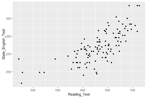
The example demonstrated in Figure 1 reveals that students who had high reading scores tended to also have high English language arts test scores. Part of the explanation for this is both tests were designed to measure similar constructs, as the English language arts test contains items that measure skills associated with general reading ability. Here we see that there was a positive relationship between the variables: where scores for one variable increased, scores for the other variable also tended to increase. This means these variables exhibited a positive correlation. There also can be negative correlations between variables in which values for one variable increase while values from the other variable tend to decrease. For example, among senior citizens, as age increases, physical dexterity tends to decrease.
The rate of the correlation between variables can be defined in a standardized way. We can have positive, zero, or negative correlations (i.e., r), with values ranging from -1 to 1. The basic guidance for interpreting the strength of the relationship based on the correlation coefficient can be seen in Table 1 (Hinkle et al., 2003). A maximum correlation value of r = 1 indicates that there is a perfect positive relationship between the two variables. In our example in Figure 1, the correlation between the two tests is 0.73, indicating a strong relationship because it is close to 1. Likewise, a correlation of r = -1 defines a perfect negative relationship between the two variables. A correlation of r = 0 means there is no relationship between the two variables.
Table 1. Guidance for Interpreting the Size of a Correlation Coefficient
| Size of Correlation | Interpretation |
|---|---|
| .90 to 1.00 or -.90 to –1.00 | Very high positive or negative correlation |
| .70 to .90 or -.70 to -.90 | High positive or negative correlation |
| .50 to .70 or -.50 to -.70 | Moderate positive or negative correlation |
| .30 to .50 or -.30 to -.50 | Low positive or negative correlation |
| .00 to .30 or .00 to -.30 | Negligible correlation |
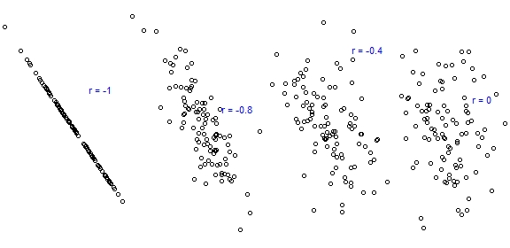
Graphing the values from the two variables in a scatterplot is always helpful to get a sense of the relationship between the variables. Figures 2 and 3 show examples of plots representing different correlation values from 1 to -1.
Figure 2. Examples of Positive Correlation
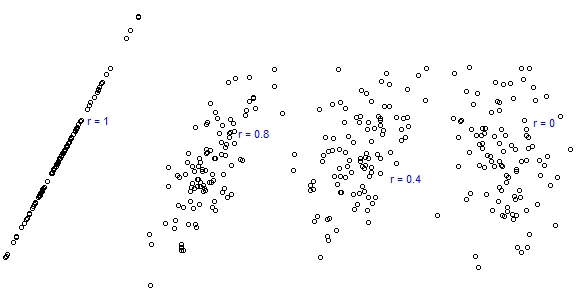
Figure 3. Examples of Negative Correlation
Considerations When Interpreting Correlations
There are certain considerations to keep in mind when interpreting correlations. Suppose we have data of two variables of a certain population. The data are plotted along the x-axis (horizontal line) and y-axis (vertical line), respectively, as shown in Figure 4. We see the trend that as x values increase, y values also increase. The correlation in this case is r = 0.8, indicating a strong positive relationship. However, suppose we consider only a subset sample of the whole population, which is indicated in yellow, and estimate the correlation for this group. In this case, we have a much lower correlation of 0.27.
Figure 4. Example of Range Restrictions
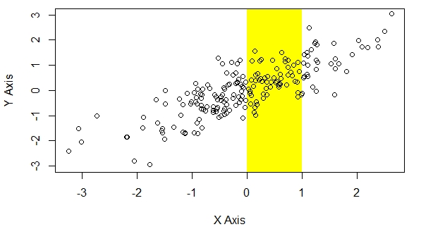
What we have here is the effect of range restriction, where looking at a subgroup of a whole sample can lead to a different interpretation of the result. Therefore, we must be mindful of the characteristics of the data when interpreting correlation coefficients. Additionally, measurement error can affect the magnitude of a correlation. Measurement error refers to the difference between the scores obtained from a measure and students’ actual abilities. Error can happen for a variety of reasons, such as problems with the delivery of directions, effort or attention of students during testing, test items, scoring process, and reporting of data. The larger the measurement error, the lower the correlation between two variables (e.g., measures of reading ability).
Avoid a Common Misconception of Correlations
A common misconception that people can make is determining that there is a causation between two variables just because there is a positive or negative correlation. As the saying goes, “Correlation does not mean causation.” An obvious example of this would be the relationship between height and reading ability. We can have data from a sample of elementary school students that show as students get taller, they are more adept at reading. However, we cannot conclude that being taller causes better reading ability when there are biological factors at play, such as students’ general maturation as they get older, and environmental factors, such as increased reading instruction and student practice over time. In order to show causation between two variables and rule out competing explanations for the observed relationship, we would need to rely on different research designs.
Correlation is a good way to describe a relationship between two phenomena, and we can interpret the strength and direction of the relationship based on the magnitude of the Pearson correlation. Graphing the relationship between the two variables also can help us get a clearer picture of the relationship between them. However, we must be mindful of potential issues, such as range restriction and measurement error, when we are intending to draw conclusions about the magnitude of the relationship. Lastly, just because there is a correlation between two events does not necessarily mean there is causation, as other factors must be considered and further statistical analysis needs to be done.
References
Allington, R. (2014). How reading volume affects both reading fluency and reading achievement. International Electronic Journal of Elementary Education, 7, 13-26. https://files.eric.ed.gov/fulltext/EJ1053794.pdf
Greaney, V. (1980). Factors related to amount and type of leisure time reading. Reading Research Quarterly, 15, 337-357. https://doi.org/10.2307/747419
Hinkle, D. E., Wiersma, W., & Jurs, S. G. (2003). Applied statistics for the behavioral sciences (5th ed.). Houghton Mifflin.
Kirsch, I., de Jong, J., Lafontaine, D., McQueen, J., Mendelovits, J., & Monseur, C. (2002). Reading for change: Performance and engagement across countries: Results from PISA 2000. Organization for Economic Co-operation and Development (OECD). https://www.oecd.org/education/school/programmeforinternationalstudentassessmentpisa/33690904.pdf