Editor’s note: This blog post is part of an ongoing series entitled “Technically Speaking.” In these posts, we write in a way that is understandable about very technical principles that we use in reading research. We want to improve busy practitioners’ and family members’ abilities to be good consumers of reading research and to deepen their understanding of how our research operates to provide the best information.
Many current assessments in education and psychology were developed and validated within the item response theory framework (IRT). Technical reports often provide the IRT analyses results as evidence for the interpretation and usage of the scores generated by the assessment (ACT, 2020). By using item response theory, testing programs can provide scores that represent or measure important student characteristics such as reading ability, attitude, or some other underlying trait, as well as assess the quality of each individual item included in the assessment. In this post, we provide some background information about these popular measurement models to help those using the assessments to better understand the information and interpret the data they obtain from the assessments.
Definition of Item Response Theory
The analysis, research, and reporting for assessments historically have focused on the overall descriptive results of the test such as the total number of test items correct for each examinee or the percentage of examinees who answered a particular item correctly. However, over time, other frameworks have been developed that provide a means to evaluate the characteristics of individual test items to see how good or bad an item is at measuring students’ abilities. Item response theory affords data analysts the opportunity to better understand the quality of each test item in terms of both its difficulty, and how well it can separate high-achieving and low-achieving students, known in statistical terms as discrimination. In addition, item response theory provides a way to estimate a student’s ability as well as other latent traits (i.e., unobservable cognitive constructs).
Item response theory is a family of statistical models which is widely used in educational measurement (Brennan & National Council on Measurement in Education, 2006). Item response theory analyzes data at an item level while addressing the relationship between examinees’ (in our case, we are talking about students) characteristics and the characteristics of items. Given what item response theory analysis provides, it has been extensively used in many measurement programs for developing item banks, constructing tests, developing adaptive test administrations, scaling, equating, standard setting, test scoring, and score reporting.
Item Response Theory Model and Item Parameters
The association of characteristics between items and students in item response theory models is expressed by the probability that a student with a particular ability gets a particular score on a particular item. Item response theory models assume that this probability increases as a student’s ability increases. For simplicity in this blog post, we will consider a single ability for each student and the particular score of an item being either 1 (correct) or 0 (incorrect). There are other models that measure multiple abilities per examinee and employ several other scoring approaches (e.g., rating scales), but those are outside the scope of this post.
Based on how many characteristics or parameters of items are captured, the item response theory model can be categorized in three ways:
- one-parameter logistic (1PL) model: involves estimating an item’s difficulty only
- two-parameter logistic (2PL) model: model involves estimating item difficulty and item discrimination
- three-parameter logistic (3PL) model: estimating item difficulty, item discrimination, and an additional parameter, pseudo guessing
Each model is explained in the following sections. Considering that 2PL is arguably the most standard model, we will explain 2PL first, followed by 3PL and 1PL.
Two-Parameter Logistic Model
The two-parameter logistic model is presented as the probability that a student with ability of θ (theta) gets an item correct, given the item’s characteristics (discrimination and difficulty). Typically, the probability increases as the student’s ability increases. Again, item discrimination in this context means how well the item can distinguish between high-achieving and low-achieving students, and it is usually denoted as a. Higher values of a mean that high-achieving students get the item correct while low-achieving students get the item incorrect. When there is no relationship between student ability and the probability of getting the item correct, a is close to 0. When low-achieving students get the item correct and high-achieving students get the item incorrect, the a value is negative, which is considered a poor characteristic for an item and rarely occurs. Item difficulty is defined as the skill level required to get an item correct. That often is determined by how commonly students get an item correct, and it is denoted as b. More difficult items have higher b values.
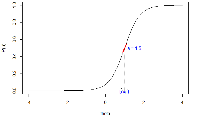
To determine how item discrimination and difficulty are related and determined statistically, we will use an example from a graph. A visual depiction of the relationship between item parameters and students’ abilities is presented in Figure 1. This plot is called an item characteristic curve (ICC). An ICC is a function that shows the relationship between ability (θ) and the probability of answering an item correctly. First, the item discrimination is represented by the steepness of the curve (in other words, the steeper the curve, the larger the item discrimination), and the maximum steepness (a) occurs when the probability of answering the item correctly (P(u)) is 0.5. Item difficulty, b, is the value of θ where this maximum steepness occurs, in other words, where the probability of getting the item correct is 0.5. In Figure 1, the curve is steepest at a = 1.5, and it occurs at b = 1, which is thus the item difficulty.
Figure 1. Item Characteristic Curve of One Item Based on a Two-Parameter Logistic Model

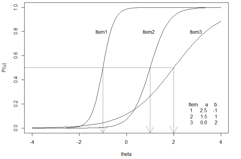
Figure 2 is a plot of the item characteristic curves for three two-parameter logistic model items, represented by the solid curves. For any given item, the probability of a correct response approaches 0 for those with very low ability levels, and the probability approaches 1 for those with very high ability levels. The dotted lines indicate the locations of θ where there is a 50% chance of getting each item correct, which are the item difficulties (b). The values of b are -1, 1, and 2 for these three items. That is, Item 3 is the most difficult item because it has the largest value, and Item 1 is the easiest item. As mentioned before, the steepest slope for each item is identified by a, which occurs on each curve where there is a 50% chance of getting that item correct. For the three items graphed in Figure 2, the a values are 2.5, 1.5, and 0.6. Based on this information, Item 1 discriminates high- and low-ability students the best because it has the highest a value of 2.5, whereas Item 3 does not discriminate high- and low-ability examinees well because its a value is 0.6.
Figure 2. Item Characteristic Curves of Three Items Based on Two-Parameter Logistic Model

Three-Parameter Model
The three-parameter logistic (3PL) model is popular because this model includes a guessing parameter in addition to item discrimination and item difficulty. Responses to multiple-choice items involve examinees guessing sometimes, so this model often fits better than a two-parameter logistic model for multiple-choice items. The guessing item parameter is denoted as c, and it is the probability that an examinee with very low ability will get the item correct due to guessing. This means that for a three-parameter logistic model, the lowest possible probability of an examinee getting the item correct is c, rather than 0 as in the two-parameter logistic model. With the 3PL model, the item discrimination (a) still represents the steepest slope. It occurs when the probability of getting the item correct is (1 + c)/2, (in other words, when the chance of getting the item correct is the average of the maximum (1) and minimum (c) possible probabilities). Similarly, the item difficulty (b) is the location of θ where the steepest slope occurs; that is, where the probability of getting the item correct is (1 + c)/2.
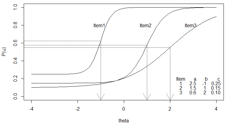
Figure 3. Item Characteristics Curves of Three Items Based on Three-Parameter Logistic Model

For example, Item 1 in Figure 3 has item discrimination a = 2.5 and item difficulty b = -1 when the probability of getting the item correct is (1 + .25)/2 = .655 because c = .25; that is, the probability of the lowest-ability students getting this item correct is .25. We can interpret these items in the 3PL model similar to how we interpreted the items in Figure 2 for the two-parameter logistic model. Item 2 in Figure 3 has item discrimination of 1.5, item difficulty of 1, and a guessing parameter of .15. This means that the probability of the lowest-ability examinees getting this item correct is 15%, suggesting this item has a moderate item discrimination and can be considered a more difficult item relative to Item 1.
One-Parameter Logistic Model
When item discrimination is fixed to a constant in the two-parameter logistic model (in other words, we assume all items have the same discrimination), we denote the model a one-parameter model. In addition, when the item discrimination is fixed to 1, some would refer to this model as the Rasch model. By fixing item discrimination to be 1, the Rasch model has several unique features from other item response theory models. More importantly, the Rasch framework allows test developers to eliminate items that do not fit a pre-specified model properly and retain other items that align properly with the pre-specified model. All details about the distinctions between the one-parameter logistic model and the Rasch model are outside of the scope of this post. However, anyone interested should consult other sources such as the research article “Rasch dichotomous model vs. One-parameter Logistic Model” written by John Michael Linacre (2005).
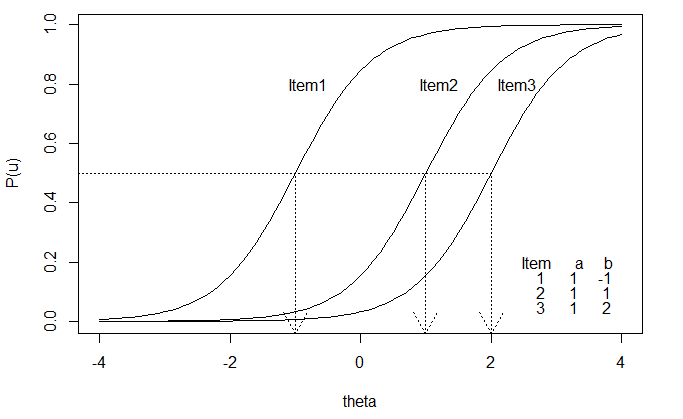
Figure 4. Item Characteristics Curves of Three Items Based on One-Parameter Model

In the one-parameter logistic model, only one item parameter is involved, which is the item difficulty (b). This is the same definition of b as in the two-parameter logistic model. The item difficulty is the location of θ where there is a 50% chance of getting the item correct. This model would be preferable when item discriminations are similar across items or when the number of parameters to estimate is very large compared to the number of students. Figure 4 shows three different one-parameter logistic item characteristic curves. A distinguishable feature in this graph is that the curves all have the same slope or steepness, which is 1. The curves have different item difficulties: -1, 1, and 2 for items 1, 2, and 3, respectively.
In summary, item response theory gives us a more flexible way of analyzing test items based on fitting a model (1PL, 2PL or 3PL), rather than simply looking at descriptive statistics on student performance. Item response theory also gives us more information on the characteristics of the items and how they relate to student responses. The characteristics of the items in item response theory are defined as item discrimination (a), item difficulty (b), and guessing (c). These characteristics of an item can be depicted in a graph called an item characteristic curve, which shows the relationship between examinee ability (θ) and the probability of examinees answering an item correctly based on their ability. A future blog post will cover more complicated item response theory models, including having more than one ability per student and more than two responses (e.g., partially correct answers, or scoring on a three- or four-point rubric scale).
References
ACT (2020). ACT Technical Manual: Version 2020.1. https://www.act.org/content/dam/act/unsecured/documents/ACT_Technical_Manual.pdf
Brennan, R. L., & National Council on Measurement in Education. (2006). Educational measurement. Praeger Publishers.
De Ayala, R. J. (2013). The theory and practice of item response theory. Guilford Publications.
Hambleton, R. K., & Jones, R. W. (1993). An NCME instructional module on: Comparison of classical test theory and item response theory and their applications to test development. Educational Measurement: Issues and Practice, 12(3), 38–47. https://doi.org/10.1111/j.1745-3992.1993.tb00543.x
Lord, F. M. (2012). Applications of item response theory to practical testing problems. Routledge.
Bond, T. G., & Fox, C. M. (2007). Applying the Rasch model: Fundamental measurement in the human sciences (2nd ed). Routledge.
Linacre, J. M. (2005). Rasch dichotomous model vs. One-parameter Logistic Model. Rasch Measurement Transactions, 19, 1032. https://www.rasch.org/rmt/rmt193h.htm
